Translation and sampling (reparameterisation) invariance of signatures

One of the big attractions of the signature transform is that it may optionally be invariant to two particular types of noise.

Translation invariance

The signature is translation invariant. That is, given some stream of data \(x_1, \ldots, x_n\) with \(x_i \in \mathbb{R}^c\), and some \(y \in \mathbb{R}^c\), then the signature of \(x_1, \ldots, x_n\) is equal to the signature of \(x_1 + y, \ldots, x_n + y\).

Sometimes this is desirable, sometimes it isn’t. If it isn’t desirable, then the simplest solution is to add a ‘basepoint’. That is, add a point \(0 \in \mathbb{R}^c\) to the start of the path. This will allow us to notice any translations, as the signature of \(0, x_1, \ldots, x_n\) and the signature of \(0, x_1 + y, \ldots, x_n + y\) will be different.

In code, this can be accomplished very easily by using the basepoint argument. Simply set it to True to add such a basepoint to the path before taking the signature:

import torch
import signatory
path = torch.rand(2, 10, 5)
sig = signatory.signature(path, 3, basepoint=True)

Sampling (reparameterisation) invariance

The signature is sampling invariant. This has a precise mathematical description in terms of reparameterisation, but the intuition is that it doesn’t matter how many times you measure the underlying path; the signature transform may be applied regardless of how long the stream of data is, or how finely it is sampled. Increasing the number of samples does not require changing anything in the mathematics or in the code. It will simply increase how well the signature of the stream of the data approximates the signature of the underlying path.

Tip

This makes the signature transform an attractive tool when dealing with missing or irregularly-sampled data.

Let’s given an explicit example.

Suppose the underlying path looks like this:

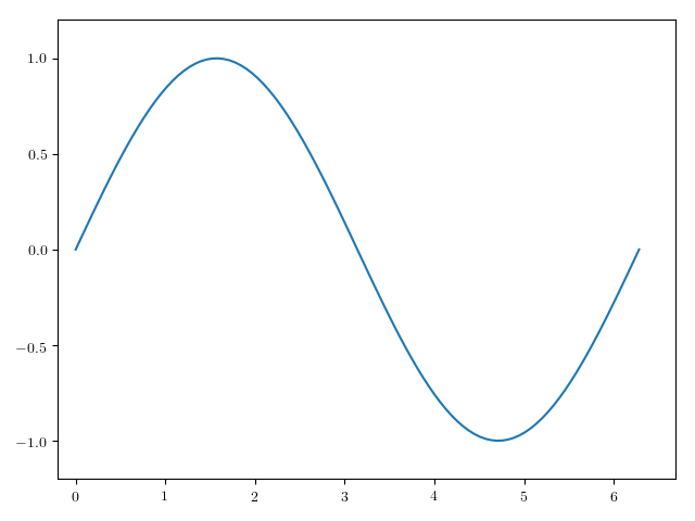
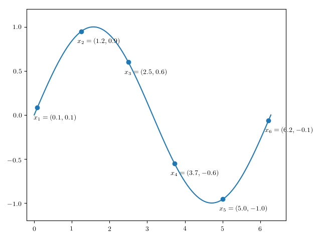
And that we observe this at particular points (the underlying path is shown as well for clarity):

Alternatively, perhaps we observed this at some other set of points:

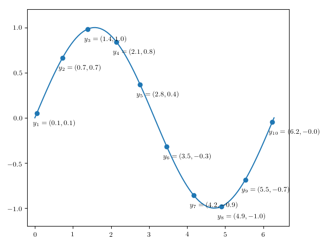
Then the signature transform of \(x_1, \ldots, x_{6}\) and \(y_1, \ldots, y_{10}\) will be approximately the same, despite the fact that the two sequences are of different lengths, and sampled at different points.

Important

The reason for this is that the index of an element in a sequence is not information that is used by the signature transform.

What this means is that if time (and things that depend on the passing of time, such as speed) is something which you expect your machine learning model to depend upon, then you must explicitly specify this in your stream of data. This is a great advantage of the signature transform: you can use your understanding of the problem at hand to decide whether or not time should be included. Contrast a recurrent neural network, where the passing of time is often implicitly specified by the index of an element in a sequence.

For example, if you want to do handwriting recognition, then you probably don’t care how fast someone wrote something: only the shape of what they wrote.